Compiling, running and analysing chains

This file is for the current release, v1.5 (June 2010).

If you are looking for older versions' read-me files, see the version history page.

Jump to:

• Compiling SuperBayeS
• Testing SuperBayes
• Running SuperBayes
• Analysing the chains and plotting (interactive plotting with SuperEGO is described here)
• Running options
• Indirect detection quantities options
• Running options for MultiNest (Nested Sampling)
• Plotting options
• Output files and contents
• Known issues

Efficiency scaling

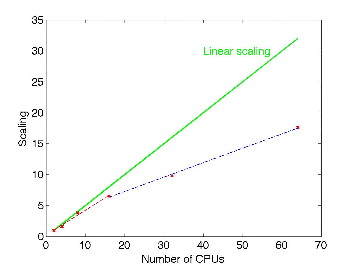The graph and the table below show the scaling of the performance of SuperBayeS with the number of CPUs used. All runs have been performed on 2.8 GHz, 1600 MHz FSB Intel processors using this ini file (log prior, all data sets included and scanning over 8 parameters, including 4 CMSSM and 4 nuisance parameters).

Each run took about 4.5 times 10E5 likelihood evaluations to gather around 50'000 samples.

From the point of view of efficiency (in terms of samples obtained per hour and per CPU) the best choice is to run with 8 CPUs. However, notice that approximate linear scaling for the inverse total time required holds up until 16 CPUs (red dashed regression line in the graph, which has slope 0.4, while perfect linear scaling would have slope 0.5, green solid line), and the efficiency gain is only moderately reduced as the number of CPUs is further increased above 16 (the blue dashed regression, with slope 0.25).

48163264

CPUs	Run time(hrs)	Samples/hour	Samples/hour/CPU	Scaling
2	176.2	284	142	1.0
117.7	444	111	1.6
46.1	1083	135	3.8
27.1	1873	117	6.5
17.9	2779	87	9.8
10.0	4952	77	17.6

Compiling SuperBayes

The code can be compiled to run on one CPU only or as an MPI code to run in parallel on an MPI cluster. In source/Makefile, turn the FC flag to mpif90 for MPI support or to ifort to work in single mode.

In MPI mode, if running MCMC the number of chains is automatically set equal to the number of processors used in the run. Each chain then produces output files with an id tag "_i", with i=1,...,n (n being the number of processors). In Grid Scan mode, the MPI mode distributes points on the grid across nodes. With MultiNest, MPI mode switches on the faster MultiNest parallel computation on the given number of nodes (recommended n=10). If MPI is off, in MCMC only one chain is produced while MultiNest runs in serial mode.

From the source directory, the command

make cleanall

cleans all the compiled files and executables. For a MPI to single processor mode transition use the command

make clean

make all

then recompiles the whole package building static libraries for each of the codes included into the package (notice that MicrOMEGAs also uses dynamical libraries). Then two binary files are produced: superbayes (which is to be used for runs in MCMC mode, postprocessing and grid scanning) and superbayes_multinest (to be used for MultiNest mode runs). The command

make superbayes (superbayes_multinest)

only recompiles files (for the corresponding mode) in the source directory. Use

make getplots

to compile the getplots routine (for chain analysis and plotting).

Testing SuperBayes

For testing purposes the testing.90 file is provided. The command

make tester

will compile it.

The run is made from the command line with the command

tester

The parameters for running the tester are hardcoded in the source\tester.f90 file, and are the same as described below. Setting debug=.true. will write the full output with detailed info about the point being considered to the file spectrum.out. By default a file called ifort.* containing the formatted output is created too. The tester works in single-point mode if test_chain = .false., otherwise it can read in a list of points from an existing chain (filename of the chain file hardcoded in tester.f90), which can be useful for testing purpose.

If your installation has been successfull, the output of running tester should match the content of the file tester.output in the main directory.

Running SuperBayeS

If MPI is turned off, Superbayes is invoked in single-processor mode from the command line with the command

superbayes (superbayes_multinest) SampleIniFile.ini

If you try e.g. to run superbayes in MultiNest mode, you will get an error message (and viceversa).

The corresponding MPI command depends on the configuration of your machine. The SampleIniFile.ini file contains all parameters for the run. Currently, only the Constrained MSSM is supported, but the package is easily customizable to extend the scan to the general MSSM if required. The syntax of the .ini file is mutuated from the CosmoMC package, and the meaning of the parameters is explained here .

SuperBayeS can be run in MCMC mode (using Metropolis-Hastings), in grid-scan mode (which returns the likelihood on a multi-dimensional grid at pre-defined spacings in parameter space) or (recommended option) in MultiNest (Nested Sampling) mode (use the superbayes_multinest binary). See running options for details.

(top)

Analysing the chains and plotting

SuperBayeS comes with GetPlots, a routine for analysing the MCMC and MultiNest outputs and plotting the results in 1, 2 and 3 dimensions. This is based on GetDist, from the CosmoMC package - refer to CosmoMC website for futher details. The current version has many extensions and new facilities that are described in detail here

GetPlots is invoked with the command (from SuperBayeS root directory)

getplots GetPlotsSample.ini

Output files are stored in subdirectories of the folder output_files folder (any pre-existing files are overwritten). Those files contain the statistical information about the run and the matlab and SuperMongo (SM) files needed to produce plots (see here for details). Data files needed by matlab and SM for the plots are stored in subdirectories of the folder plot_data (it should usually not be necessary to edit or otherwise change these files).

To generate .ps plots, go to the output_files/rootname directory and call SM (for 1D plots) with the command

sm < rootname_1D.sm

or matlab via the command

matlab < rootname_1D.m or matlab < rootname_2D.m or matlab < rootname_3D.m

Details of the format of the ensuing plots (line colours, thickness, labels, colormaps, etc) can be custom-edited in the source files source\matlab.f90 (matlab plots) and source\smplots.f90 (SM plots).

Analysis and plotting options are explained here. Interactive plotting with SuperEGO is described here.

The list of output files and their meaning is explained here.

(top)

Running options (indirect detection quantities options are listed separately here. MultiNest specific running options are here )

• file_root: the and location (and prefix) of the output files produced. The list of file produced depends on the running mode, see here . When postprocessing, this becomes the name of the input chains. If restart = T, the job restarts from the last line of the chains or from the last sampling step for MultiNest. If MCMC/MultiNest chains with the same name already exist, they are overwritten. In MCMC mode only, to prevent the overwriting from happening, set the variable FailSafeOn = .true. (hardcoded) in source/utils.F90

• out_root: the name of the output files produced when postprocessing (otherwise ignored).

• restart_and_continue: set it to F to start a new job, set it to T to continue from where a previous chain stopped. In MultiNest mode, don't change nlive option while restarting a run otherwise the program would abort.

• action: determines how the scanning is performed:

  • action = 0 to do MCMC (currently only Metropolis-Hastings is supported). Set the lambda parameter to a value > 0 to activate the bank sampling mode. If lambda > 0 it is assumed that a bank samples file exists with name file_root_bank.txt .

  • action = 1 to post-process an existing set of chains (useful for computing new variables, or doing a rough posterior adjustment for new data or new priors without re-running the whole chain, or for computing the indirect detection quantities corresponding to the output of a MCMC or MultiNest run)

  • action = 4 to compute the likelihood on a fixed-grid in parameter space (if MPI is enabled, each chain covers one part of the grid). When run in grid-scanning mode, only physically admissible points (e.g., EWSB achieved, no tachyonic masses, etc) are saved.

  • action = 5 for MultiNest (recommended)

• When post-processing, redo_like = T will recompute the likelihood from the saved values of the variables in the chains, without recomputing the theory. This is useful if only the data have changed, but you must have saved all of the relevant variables in the chains, as observables are not recomputed. redo_theory = T will recompute the observables, as well (useful if the theoretical predictions have changed). redo_change_like_only = T will just change the likelihood (i.e., multiplicity of the samples is not affected. NB: this is not recommended except for testing purposes).

• skip_lines: number of samples that are not saved at the beginning of the MCMC run (burn-in period). You might as well save them and remove them later when analysing the chains.

• Use_MICRO: set it to T uses MicrOMEGAs for computing the relic density of dark matter abundance. Otherwise DarkSusy is used instead. Notice that currently dark matter direct and indirect detection quantities are computed by DarkSusy anyway.

• compute_xxx: those flags determine which quantities are computed and saved in the .txt files:

  • compute_DM: set it to T to compute the relic dark matter abundance. CDM_purely_LSP = T assumes the LSP is the dark matter, otherwise the dark matter is made up of LSP plus another component and hence the WMAP3 observations are only an upper bound (the latter mode is currently untested).

  • compute_Direct_Detection : set it to T to compute direct detection cross sections.

  • compute_Indirect_Detection: set it to T to compute indirect detection quantities.

  • compute_Collider_Predictions: set it to T to compute collider-related quantities (masses, etc).

  • compute_BD: set it to T to compute B decay predictions.

  • compute_FH: set it to T to compute cross sections and branching ratios using FeynHiggs. Customize the variables you want to save by modifying the routine ReduceOutput in source/paramdef.f90 and the corresponding type, Reduced_Out

• feedback: controls amount of text printed on standard output. 0 = none, 1 = some, >2 debug mode.

• use_xxx: those flags determine which quantities are used in the computation of the likelihood (obviously if you want to use them you have to set the relative compute_xxx flag to T). All of the data values are found in the file likedata.f90. Refer to our paper for how the likelihood is computed. Meaning as below.

• Use_Nuisance: set it to T to use current constraints for nuisance (SM) parameters.

• Use_CDM: set it to T to use current cosmological constraints on dark matter abundance.

• Use_LEP: set it to T to use constraints from LEP on sparticle masses and Higgs mass.

• Use_Anomalous_Mu: set it to T to use constraints on the anomalous magnetic moment of the muon.

• Use_bsgamma: set it to T to use constraints on the process B-> s gamma.

• Use_Bsmumu: set it to T to use constraints on the process B-> mu mu.

• Use_Mass_W: set it to T to use constraints on the W mass.

• Use_Weak_Mixing_Angle: set it to T to use constraints on the effective weak mixing angle.

• Use_Delta_MBs: set it to T to use constraints on Bs-Bs oscillations.

• Use_Butaunu: set it to T to use constraints on the process B-> nu tau.

• Use_DD: set it to T to use constraints on direct dark matter detection (currently not supported).

• Use_ID: set it to T to use constraints on indirect dark matter detection methods (currently not supported).

• use_data: select from the list to use current data (Jan 2010) or constraints from future observations (edit your future data in source/likedata.f90).

• propose_matrix: set it to the name of the file containing the covariance matrix from previous runs. Used to adjust the proposal width in the new run (MCMC only).

• redo_likeoffset: when postprocessing it might be useful to put an offset to the loglike if there is a large change to it with new data to get sensible weights.

• samples: number of samples to obtain per chain (MCMC only). All accepted samples are counted (after burn-in). If in grid-mode, this sets a limit to the maximum grid points per chain that will be allowed - increase it as needed.

• temperature: temperature of the MCMC (1 by default). Increase to explore the tails, jump more easily to disconnected regions of parameter space, etc (must be matched by the cooling factor when analysing the chains).

• rand_seed: if blank this is set from system clock.

• use_log: whether to use a log scale (set it to T) or a linear scale (set it to F) for the gaugino and scalar mass parameters.

• param_xxx: parameters over which to do the scanning. For MCMC and MultiNest, flat priors are taken on this set of parameters. The meaning of the 5 real numbers is the following:

  • For MCMC: start_central_val, min_val, max_val, start_width, propose_width

    where start_central_val is the central value around which the chain is started, min_val/max_val are the minimum and maximum values allowed (prior range), start_width is the standard deviation around start_central_val from which the starting point is drawn, propose_width is the proposal width for the Metropolis-Hastings step (overriden if a covariance matrix is present).

  • For grid scanning: ignored, min_val, max_val, ignored, grid_step

    where ignored is irrelevant, min_val/max_val set the grid's boundaries and grid_step gives the step size in that direction. The grid is split among chains if running in MPI mode. If the number of grid points per chain exceeds the number of samples, you will be asked to increase samples.

  • For MultiNest: ignored, min_val, max_val, ignored, ignored

    where ignored is irrelevant, min_val/max_val set the ranges of the priors The number of samples is automatically determined by the tolerance level requested for the evidence value.

(top)

Indirect detection quantities options

All of the following options are only relevant if compute_Indirect_Detection is set to true. We recommend using the post-processing routine to compute indirect detection quantities from the saved MCMC or MultiNest run rather than computing them directly in the run.

• compute_ID_gadiff: set it to T to compute the differential spectrum of gamma-ray.

• compute_ID_gacont: set it to T to compute the gamma-ray flux with continuum energy spectrum integrated above some threshold energy.

• compute_ID_gamonoc: set it to T to compute the monocromatic monochromatic gamma-ray flux induced by 1-loop annihilationprocesses into a 2-body final state containing a photon. There are two such final states: the 2 photon final state and the final state with a photon and a Z boson.

• compute_ID_antiprot: set it to T to compute the differential spectrum of antiprotons.

• compute_ID_antideut: set it to T to compute the differential spectrum of antideutrons.

• compute_ID_posit: set it to T to compute the rates of positrons.

• compute_ID_positfrac: set it to T to compute the positron fraction.

• compute_ID_muonsun: set it to T to compute the total rates in neutrino telescopes from the Sun above some threshold energy.

• compute_ID_muonearth: set it to T to compute the total rates in neutrino telescopes from the Earth above some threshold energy.

• compute_ID_sundiff: set it to T to compute the differential rates in neutrino telescopes from the Sun.

• compute_ID_muonearthdiff: set it to T to compute the differential rates in neutrino telescopes from the Earth.

• compute_ID_eqbsun: set it to T to compute the capture and annihilation rates of neutralinos at Sun.

• compute_ID_eqbea: set it to T to compute the capture and annihilation rates of neutralinos at Earth.

• compute_ID_musuevent: set it to T to compute the number of events produced at ICECUBE from neutralinos annihilation to neutrinos at Sun.

• compute_ID_muonhalo: set it to T to compute the total rates in neutrino telescopes from the halo above some threshold energy.

• compute_ID_muonhalodiff: set it to T to compute differential rates in neutrino telescopes from the halo.

• compute_ID_sigmav: set it to T to compute the annihilation cross section sigma v at p=0 for neutralino-neutralino annihilation.

• compute_ID_efluxes: set it to T to compute differential fluxes over a range of energies for each model. It only works in the postprocessing mode.

• num_hm: sets the number of halo profiles used.

• modelxx: sets the specific halo models you want to use (see DarkSusy).

• pbmodel: sets the antiprotons and antideutrons propagation model one wants to use (see DarkSusy).

• epmodel: sets the positron diffusion model (see DarkSusy).

• ntmodel: sets the neutrino telescopes parameters (see DarkSusy).

• cospsi0: for gamma-rays and neutrinos with the chosen halo profile, sets the line of sight integration factor j in the direction of observation, which is defined as the direction which forms an angle psi0 with respect to the direction of the galactic centre (see the .ini file).

• delta_gamma: for gamma-rays if one takes into account the angular resolution of the detector then delta_gamma is set is given (in sr) otherwise it is set to 0 (see the .ini file).

• egam: sets the energy (GeV) for the differential gamma-ray flux.

• egath: sets the threshold energy (GeV) for the gamma-ray flux with continuum energy spectrum.

• BF: sets the boost factor for antimatter fluxes.

• epb: sets the kinetic energy (GeV) of the antiprotons for the differential flux of antiprotons.

• edb: sets the kinetic energy (GeV) of the antideutrons for the differential flux of antideutrons.

• eep: sets the kinetic energy (GeV) of the positrons for the differential flux of positrons.

• eth: sets the energy threshold (GeV) for neutrino telescopes.

• thmax: sets the maximum half-aperture angle (degrees) for neutrino telescopes.

• enu: sets the neutrino energy (GeV) for differential flux of neutrinos.

• theta: sets the angle from center of Earth/Sun in degrees for neutrino telescopes.

• rtype: sets the type of fluxes (see the .ini file).

• delta_nt: as delta_gamma for neutrino fluxes.

• exposure: sets the exposure time (yrs) for the computation of events at ICECUBE.

• ic_config: sets the ICECUBE string configuration for the computation of events (see the .ini file).

• efluxes_i: sets the initial energy of the fluxes spectrum computation once the compute_ID_efluxes is on.

• efluxes_f: sets the final energy of the fluxes spectrum computation once the compute_ID_efluxes is on.

• nbins: sets the number of the bins to be scanned in the fluxes spectrum computation. Notice that it is in logaritmic scale.

Running options for MultiNest

• multimodal: whether to produce separate statistics and samples for each found mode. For problems with several modes with vastly different amplitudes, setting multimodal to T stops live points from migrataing to dominant modes from weaker modes and therefore allows all the modes to be explored at greater depth. If the problem is inherently multi-modal but multimodal is set to F, the sampling is still done from all the modes but only the modes contributing significantly to the evidence are explored in any detail.

• maxmodes: the maximum number of modes expected. This is relevant only if multimodal = T and is used for memory allocation only. If more modes are found than maxmodes then the program would abort with the error message "ERROR: More modes found than allowed memory. Increase maxmodes in the call to nestrun and run MultiNest again. Aborting". The user can then resume the sampling by setting maxmodes to a higher value and running SuperBayeS again with restart_and_continue set to T.

• nCdims: no. of parameters for mode separation. This is relevant only if multimodal = T. Mode separation is done through a clustering algorithm. Mode separation can be done on all the parameters (in which case nCdims should be set to ndims, the total no. of sampling parameters) & it can also be done on a subset of parameters (in which case nCdims < ndims) which might be advantageous as clustering is less accurate as the dimensionality increases. If nCdims < ndims then mode separation is done on the first nCdims parameters. For CMSSM, the recommended value is 2 (with mode separation being done on m_0 and m_{1/2}).

• ceff: whether to run MultiNest in constant efficiency. If ceff is set to T, then the enlargement factor of the bounding ellipsoids are tuned so that the sampling efficiency is as close to the target efficiency (set by eff) as possible. This does mean however, that the evidence value may not be accurate.

• nlive: the total no. of live points. The recommended values are as follows (see 1101.3296 for details):

  • For an accurate mapping of the Bayesian posterior, nlive = 4000 .
  • For an accurate computation of the Bayesian evidence, nlive = 4000 .
  • For an accurate mapping of the profile likelihood, nlive = 20000 .

• eff: the maximum sampling efficiency. A value greater than 1 means that the MultiNest will sample from a region with volume smaller than the volume enclosed by the prior volume at any given iteration. The recommended values for parameter estimation & model selection are 2.0 & 1.0 respectively. If running in constant efficiency mode (i.e. when ceff = T), eff is the target efficiency and its recommended value is 0.1 or lower.

• tol: defines the stopping criteria. The recommended values are as follows (see 1101.3296 for details):

  • For an accurate mapping of the Bayesian posterior, tol = 0.5 .
  • For an accurate computation of the Bayesian evidence, tol = 0.5 .
  • For an accurate mapping of the profile likelihood, tol = 0.0001 .

(top)

Plotting options for getplots

Plotting options are set in the GetPlotsSample.ini file to be used with getplots as follows:

• file_root: name of chains to be analyzed (including chains subdirectory). Numbering of chains set automatically using the chain_num setting.

• out_root: name of output files (if empty, the same as file_root)

• add_columns: number of new combinations of variables to add to the anaylsis. Customize this by writing your own AddParams routine in GetPlots.f90

• smoothing: set to T to use Gaussian smoothing with a kernel about 3 bins wide. Useful to reduce jaggedness of 2D contours. Set it to F to use top-hat bins (no smoothing).

• chain_num: number of chains to process. If 0 it assumes one chain and no filename suffixes. The code automatically looks for MultiNest output if it does not find an MCMC chain.

• first_chain: default is 1.

• exclude_chain: if you want to exclude one particular chain from the analysis.

• num_bins: number of bins per dimension.

• skip_bin: number of bins to discard at the edges (use with care).

• ignore_rows: number of rows to discard when analysing (burn-in period. Note this should be used only with MCMC-generated chains. MultiNest does not do any burn-in and therefore no rows should be discarded).

• cool: cooling factor, must match the temperature of the chain (default 1. MCMC only).

• thin_factor: set it to produce a file_root_thin.txt file containing every thin_factorth sample (MCMC only. Usually, not needed with MultiNest).

• thin_cool: cooling factor applied in the thin process. It has to match the temperature of the chain (default 1).

• adjust priors: performs rough importance sampling. Write your own AdjustPriors routine.

• map_params: set it to T to map chain parameters to any function of the parameters (e.g, transform from linear to log scale for plotting. This will not adjust the prior, though! use adjust_priors instead). Write your own MapParameters routine.

• contour1, contour2: percentage of confidence levels contours.

• force_twotail: set it to T to force 2-tails limits on all variables regardless of the settings for tailsxxx below.

---

• plotparams_num: how many variables to get plots for. If zero, uses all parameters which have labels in .info file plus all added parameters (with labels labAxxx). This setting can be exceedingly slow, so use with care.

• plotparams: list of parameter numbers to plot, must match plotparams_num above. For the parameters saved in the chain, look at the .info file to determine which number corresponds to which parameter. For added parameters, use the syntax A1, A2, ..., where a capital A denotes that the number refers to an added parameter (numbering for added parameters goes from 1 up to the maximum determined by the value in add_columns).

• plot_1D_pdf: set to T to plot the 1D Bayesian posterior pdf.

• plot_1D_meanlike: set to T to plot the 1D mean likelihood (mean is taken over the posterior). Notice this is only plotted in the 1D SM files (not in the 1D Matlab).

• plot_1D_meanchisq: set to T to plot the 1D mean chi-square. Notice this is only plotted in the 1D SM files (not in the 1D Matlab).

• plot_1D_profile: set to T to plot the 1D profile likelihood (both with SM and with Matlab)

• plot_1D_likelihood: set to T to plot the 1D likelihood from the data when plotting the observables (such as the DM relic abundance, g-2, etc). The codes determines automatically which variables have an associated likelihood function and takes the values from the likedata.f90 file.

---

• plot_2D_param: set it to 0 to produce 2D plots only of a list of parameters combinations (specified below). Set it to the number corresponding to the parameter you want to have 2D plots of (plotted against all other parameters that have labels).

• plot_2D_num: number of parameters combinations for which to produce a 2D plot (mean quality of fit and marginal probability density will be both plotted by default and saved in different .ps files). Only relevant if plot_2D_param = 0. You must then specify a list of plot1, plot2, ... giving the couples of parameters that you want to plot against each other. Use A to denote added variables, same syntax as above.

• plot_contours: set to T to plot contours in 2D plots. Contours will be plotted for the posterior pdf and the profile likelihood, following the levels for the 2 statistics.

• plot_mean: set to T to plot the posterior mean in the 1D (as a vertical bar) and 2D plots (as a solid dot).

• plot_bestfit: set to T to plot the best fit value in the 1D (as a cross) and 2D plots (as a cross with a circle around it).

• plot_reference: set to T to plot a reference point of your choosing (hardcoded in the subroutine DefineRefPoint in mcsamples.f90. Plotted as a diamond.

• plot_2D_meanlike: set to T to plot the mean likelihood in 2D.

• plot_2D_meanchisq: set to T to plot the average chi-square in 2D.

• color_scheme: color_scheme type for 2D plots. Options are: 1 for a smooth, continous colorscheme (default) or 2 for a discrete colour scheme with solid colouring of the contours.

• all_2D_plots: set it to T if you want to produce plotting data files for all possible 2D combinations (although the ones that will be included in the .m file are still controlled by the plot_2D_num variable above). This is useful if you want to plot some other parameter combination subsequently without having to re-run GetPlots to get the corresponding matlab file. Careful, setting this to T can produce several thousands of plot files.

• colorbar_on: set to T to add a colorbar to the bottom of 2D files.

---

• num_3D_plots: number of 3D scatter plots to produce. You must then specify a list of 3D_plot1, 3D_plot2, ... giving the triplets of parameters that you want to plot (x axis, y axis and coloured variable). Use A to denote added variables, same syntax as above.

• do_3D_plots: set it to T to produce a single samples file used by 3D plots. Setting is overriden to T if num_3D_plots > 0.

• colormap_name: put here the name of the colormap you want to use for 3D plots. see colormaps/ directory. If empty, uses default 'jet' colormap.

---

• labA1, labA2: labels for added parameters. Parameters saved in the chain automatically get their labels from the .info file.

• limitsxx: lower and upper limit for the 1D binning. Samples below/above the limits are put in the first/last bin. Use limitsA1, limitsA2, ... for added variables instead. If you only want to adjust the limits of the 1D plot, use plot_limits instead.

• plot_limitsxx: lower and upper limit in the 1D and 2D plots of the corresponding variable (purely cosmetic, does not affect the statistics).

• tailsxxx: set to 1 for 1-tail probabilities and to 2 for 2-tails (default). For added variables use tailsA1, tailsA2, ... instead. Overridden if force_twotail = T.

---

• cov_matrix_dimension: number of parameters to get covariance matrix for. If you are going to use the output as a proposal density make sure you have map_params= F, and the dimension equal to the number of MCMC parameters of the run (9 for the CMSSM).

(top)

List of output files and their content

• Output files from MCMC runs: those files are in the outroot directory.

  • .txt MCMC chains

  • .log log file containing details of acceptance ratio and useful timing information if timing=.true. in source/paramdef.f90)

  • .info a file containing the name and position of the saved variables and other details of the run

• Output files from MultiNest runs:

  • .txt the chains (posterior samples) produced by MultiNest. This file is updated after every 100 iterations.

  • equal_weights.dat updated after every 1000 iterations & contains the equally weighted posterior samples.

  • phys_live.points the current set of live points. This file is updated after every 100 iterations.

  • stats.dat contains the Bayesian evidence, mean, max likelihood & MAP parameters. If multimodal = T, it will contain local evidence values and mean, max likelihood & MAP parameters for each found mode separately. This file is update after every 1000 iterations

  • resume.dat contains the information about check-pointing.

  • post_separate.dat is created only created if multimodal = T. It contains the chains (posterior samples) for modes with local log-evidence value, separated by 2 blank lines. Format is the same as .txt file.

• Output files from getplots:

  • .margestats marginalized 1D statistics for the Bayesian posterior. Posterior mean point.

  • .likestats 1D statistics for the mean quality of fit. Best fit point.

  • .proflstats 1D statistics for the profile likelihood.

  • _1D.sm generates 1D plots with SM.

  • _1D.m generates 1D plots with matlab.

  • _2D.m generates 2D plots with matlab.

  • _3D.m generates 3D plots with matlab.

  • .burnin.sm generates a burn-in plot for MCMC chains with SM (useful for MCMC diagnostics).

  • .chain_loc.sm generates with SM a plot showing the location of the chain in parameter space as a function of step number (useful for MCMC diagnostics).

(top)

Known issues